Home Science Page Data Stream Momentum Directionals Root Beings The Experiment
Before going on, let us get a grip on the reins of this wild Data Stream. In attempting to characterize our Data Stream with central tendencies, we discovered that the Decaying Average, based upon a contextual equation rooted in decay, was both a sensitive and relevant measure and easy to compute. We then suggested that this type of measure could have provided an evolutionary advantage to early humans. Further the neural networks posited by scientists of the brain were an easy physiological way that animals could have performed these computations. We will use the neural network metaphor in the Deviation discussion that follows. {See Boredom Principle Notebook for more on Neural Notebooks.}
Let us look back at our Data Stream and try to characterize it in another way. We want to know how much it changes, its potential for variation, Initially we just 'remember' the highest and the lowest data points. This is easy. We just leave a little trace pattern where the highest and lowest data points came in. These points determine the Upper and Lower Limits of Possibility. If new data comes in that is higher or lower than these limits, it replaces them. While these upper and lower limits are crucial in characterizing our Data Stream, they are not enough, as we shall see from the following example.
A new restaurant opens. The Data Stream in question is the number of customers the restaurant serves each night. The job of the manager is to predict how much staff to schedule in order to service the anticipated number of customers. His ability to predict from the Data Stream is crucial to the financial vitality of the business. Too much staff means high labor costs; not enough staff means customer complaints. It is busier than they expect the first week; they get service complaints. Our manager doesn't want this to happen again and so staffs according to the Upper Limit of Possibility generated in the first week of business. Business dips after the first rush of curiosity seekers but the staff remains the same because staffing is based upon the upper possible limit. There are no customer complaints but when the owner receives his first profit and loss statement, he shrieks because his labor costs ate up all of his profits. He says his labor costs will drive him out of business. He hires a new restaurant manager to bring labor costs down. The new manager makes an average of the number of customers coming in on a nightly level and schedules his staff according to these averages. He begins having lots of complaints on the nights when the number of customers far exceeds the average. His business drops, the averages drop, the staffing drops. The complaints continue, the business drops, the averages drop, the staffing drops, and so forth until one unfit business closes its doors. The first manager based his decisions on the range of possibility. This killed the labor cost. The second manager based his staffing on the averages, which saved the labor cost but killed his service, and inevitably his business.
Although knowledge of a Running Average and a Range is useful, it is not enough to run a fit business. More information is needed. Although occasionally there is a burst of customers, which overwhelms the short-staffed waiters, the manager can't continually staff for the busiest night because his labor costs will eat him up. Additionally he can't just staff for the average night because his service will suffer on randomly busier nights. A middle ground is necessary. To stay in business, the manager must staff his restaurant with enough personnel to please most of the people most of the time, without sending his labor costs through the roof.
Although the manager must be aware of the upper and lower limit of possibility, he must be equally aware, if not more so, of the upper and lower limits of probability. The upper and lower limits are easy to remember; no calculation is necessary. Running averages are a little more complicated. Calculating the upper and lower limits of probability is another story.
Governing a life by the range of possibilities is paralyzing. Almost anything good or bad can happen, so the conclusion is reached to stay at home to protect the species from all the bad that can happen. Governing an existence by averages is stagnating, repeating the same process over and over because it worked before. Governing a life by the range of probabilities is liberating because it minimizes the possibility of the extremes, but gives a range of effective responses.
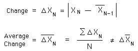
How are the limits of probability calculated? The first way would be to subtract the new data bit from the old average and then to store and average the differences. Symbolically represented as:
Note that the average change is not the same as the change in averages dealt with in the notebook Data Stream Momentum.
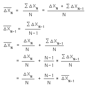
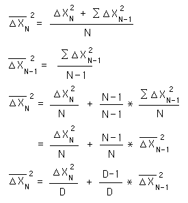
As mentioned before summations are a bear of a calculation. So we will first convert the summation into a simple sum based upon the past average change, the number of samples, and the new change.
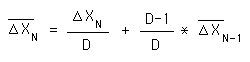
Because the above equation uses N, the number of samples, which maximizes the past and minimizing the present, contrary to the needs of a Live Set, we will convert to the N to a D, the Decay Factor. This style retains more relevant data, is more sensitive to changes in the data flow, and also lends itself to experimentation as mentioned above. So our defining equation for the average change reads:
This is an accurate description of an arithmetic distribution, where the Data Stream distributes itself over an arithmetic range, i.e. extreme values are still within the arithmetic distribution.
In nature many times the distribution is over a geometric or exponential scale. Earthquakes are the classic example, where moving up one on the Richter Scale for earthquakes multiplies the power by ten. Squaring the differences is a way of stretching our scale so that the average change will accommodate more of the extreme data. Squaring the differences reflects the geometric distribution. Symbolically and algebraically these differences are worked out below.
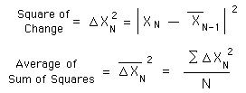
First we turn the very difficult summation of squares into a sum of relevant information. Then we eliminate the irrelevant number of samples, N, replacing it with a Decay Factor, D, as before.
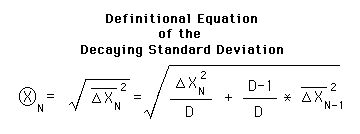
The square of the average changes is called the variance. But we want a number, which relates to our Data Stream. Therefore we must take the square root of our variance to get a number with relevance to our Data Stream. This is called the Standard Deviation. Our version is called the Decaying Standard Deviation because it is based upon Decaying Averages and Decaying Differences. Below is the defining definition of the Decaying Standard Deviation.
The preceding was not a proof. It has only been a demonstration as to why this definition was chosen. We are not saying that this is true because of the algebra. We are saying that we have chosen to define this quantity in the way we have because of the preceding demonstration and justification.
Below is a chart, which compares the arithmetic and geometric interpretations of Average Changes. The gray mass represents the actual Data Points for Exercise. The Blue Line is the Decaying Average, D= 12. The Red and Green Lines are 2 Arithmetic Deviations from the Average. The Gray and Pink Line are 2 Geometric Deviations from the Average.
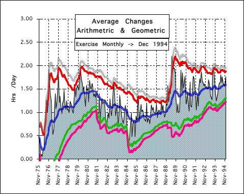
One, note how closely the Arithmetic and Geometric Deviations mirror each other. Two, note that the Arithmetic Deviation is always less than the Geometric Deviation. Finally, note that both are good predictors of the Realm of Probability, i.e. almost all the Data falls within 2 Deviations of the Decaying Average.
The measure of the limits of probability is a very useful. With unlimited resources, tuning the organism to the limits of possibility is best. However most organisms are limited by time and energy and so need to tune themselves to the realm of probability rather than the range of possibility in order to conserve precious resources. It is always possible that a predator might catch a quick prey but the predator would expend a lot of energy and might still be unsuccessful. So the predator doesn't waste his energy on the quickest prey but instead focuses upon the old, weak, or young where his probabilities are much higher. With limited resources the focus must shift from the possible to the probable to facilitate long-term survival.
The limits of possibility are easy to discover. How are the limits of probability computed? We've discovered a Geometric and Arithmetic Deviation, which yields the limits of probability. The Geometric Deviation computation involves square roots, which seems a bit complicated for the average caveman, fish, or dinosaur. The Arithmetic Deviation is much simpler. An averaging mechanism has already been set up to calculate the Decaying Average.
Set up another neural network to average the Average Changes. This average is called the Average Difference or Deviation. The organism has already set up a neural network to compute a Running Average. This computation needed the difference between the new Data Bit and the old average. Instead of throwing that difference away, use it to set up a Running Average of Differences. Take the new Difference compare it to the old Average Difference. If it is larger, then add a little to the Old Average; if it is smaller, then subtract a little; if it is the same, then the Average Difference remains the same. The Running Average plus or minus double the Average Difference yields the Realm of Probability. Remember this is not the Range of Possibility.
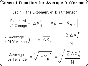
How much do we to add or subtract from our Average Difference? When we were calculating the Decaying Average, our caveman varied D, the Decay Factor, to tune up his predictions. With an Arithmetic Range this would work again. However if the Range is exponential then the exponent of change needs to be set higher than one to accommodate more extreme values in its predictions.
When r, the exponent of distribution, is equal to 1, then the Average Difference or Deviation is the Average Arithmetic Difference. This exponent reflects an arithmetic Range. When r, the exponent of distribution, is equal to 2, then the Average Difference is the Standard Deviation. This exponent reflects a Geometric Range. The truth for each Data Stream is probably somewhere in between. Each Data Stream would have a different exponent of change, which would have to be established experientially, experimentally.
What is he measuring? He could certainly care less about the exponent of distribution. What he does care about is containing the Realm of Probability. If he can get a tight reign on the Realm then he can save much crucial energy needed for survival. He also can afford to extend himself beyond normal limits because of precise knowledge of the Realm. "It normally takes me about 3 hours to get home plus or minus an hour. The sun will set in about 4 hours. I want to be home before dark. Therefore I can stay out a little longer hunting and exploring." If our caveman's estimates are off, then he will either be home early, wasting precious hunting time, or he will arrive home after dark and risk being eaten. Either of the poor predictions minimizes his long-term chances for survival.
Animals and early humans needed and learned to be able to make quick predictions in flight to avoid being consumed. There are many situations but we will talk about jumping over a crevice. The predator is pursuing. The caveman comes to a crevasse. Can he jump across? It is a little beyond his Average broad jumping ability. Of course it is possible to jump across the crevasse if all factors are perfect, but is it probable? There are other means of escape, which might be more probable than this leap. If our caveman has been doing his average differences he realizes it is just beyond the realm of probable and takes another more probable escape route. If he's young and impetuous, he makes the attempt, fails, and never passes on those genes that weren't so good at computation.
This type of scenario regularly occurs with different variations in any animal, whether prehistoric or modern. "How fast can I go and still make that turn? Can I jump onto the table? What are the risks and advantages of this investment?" The ability to predict and narrow the Realm of Probability is a major evolutionary advantage. The caveman generates an internal distribution graph and cares nothing about the exponent of distribution. But the bright caveman does stretch his data exponentially to accommodate experience. Scientists, however, like consistency for comparison. This experimenter will generally choose '1' as the exponent of change. If the Data is spread out exponentially, then the exponent will be '2' which will be noted.